RAG end to end: Input, Retriever, and Generator explained
A dense overview of RAG (Retrieval-Augmented Generation): what it is, why it matters, what Retrieval, Augmented, and Generation mean, the offline ingestion pipeline, the online query flow, embeddings, cosine similarity, HNSW, and chunking.
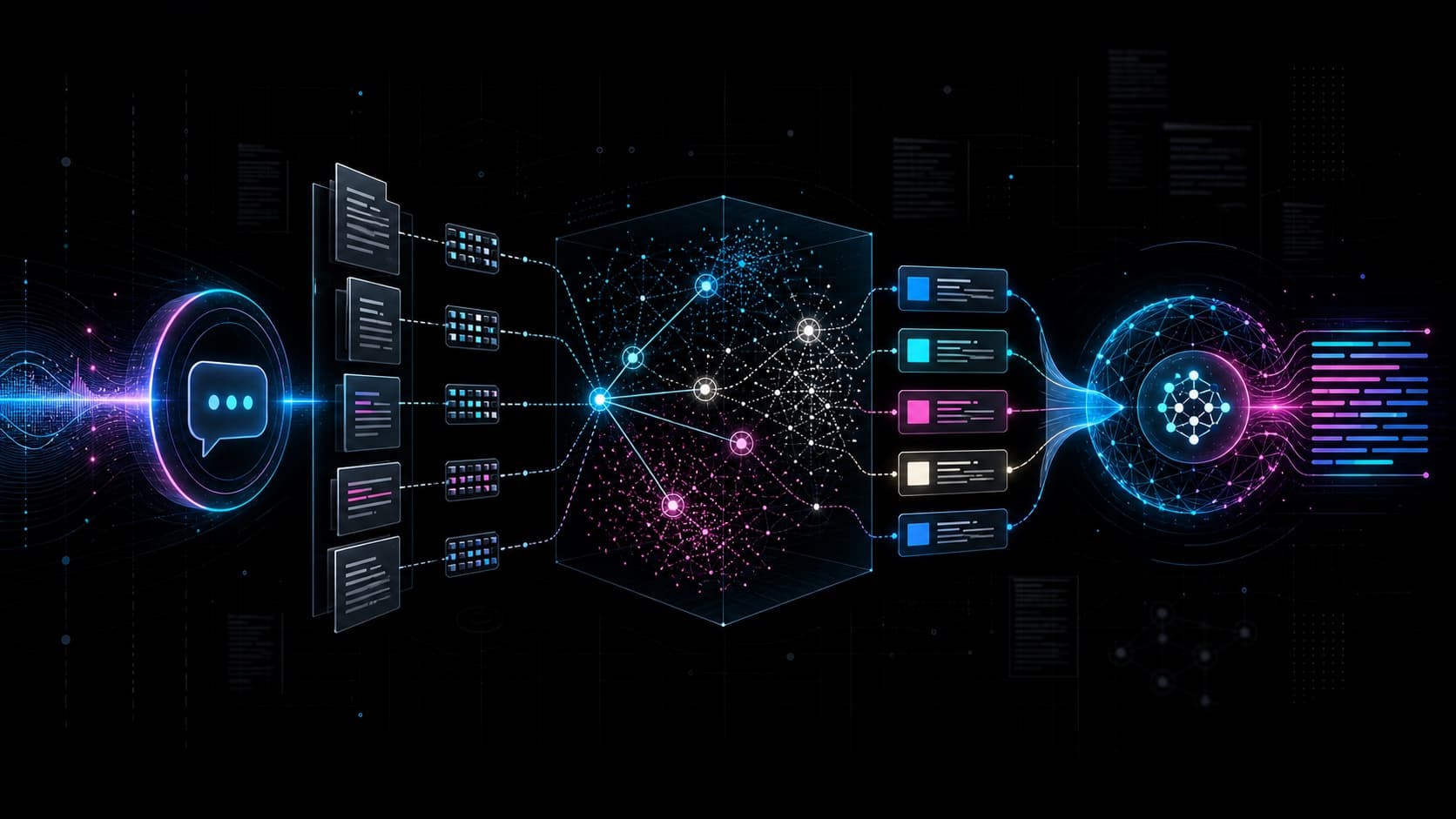
🧪 Interactive companion: this post has Canvas animations embedded — RAG flow, cosine, HNSW, and chunking. Play with them inline. Or open the lab full screen.
LLMs write fluently. But ask them about your internal PDF, your store refund policy, or anything that happened after the period the model was trained on, and they do one of two things:
- say they don't know;
- invent a confident-sounding answer with a face of truth — hallucination.
RAG (Retrieval-Augmented Generation) exists to fix this. It doesn't replace the LLM, it complements it: it adds a retrieval step before generation so the model answers by consulting real evidence instead of just "remembering" from training.
This post is a dense end-to-end overview of RAG — what it is, why it matters, what each letter means, the minimal architecture, the offline ingestion pipeline, the online query flow, and the concepts that hold it all together (embeddings, cosine similarity, HNSW, chunking).
The one-line definition
RAG = retrieve relevant evidence chunks from a corpus + hand them to the LLM as context so it can write the answer.
Everything below is technical detail on top of that one sentence.
What R, A, and G mean
The name is literal: each letter maps to a responsibility in the flow.
Find the most relevant evidence chunks from an external knowledge base: docs, pages, tickets, PDFs, or internal data.
Attach those chunks to the prompt so the model has evidence available before answering.
The LLM writes the final answer using the user question plus the retrieved context.
Without R, the model answers only from training or from the prompt. Without A, retrieval does not become useful context for the LLM. Without G, you have relevant documents, but not yet a synthesized answer.
Why RAG exists — what each half can't solve alone
A pure LLM has two hard limits:
- It only knows what it saw during training. It has no access to private documents, recent data, or your company's internal knowledge base. Anything added later is outside the model's memory.
- It fills gaps when context is missing. If the answer depends on information that is not in the prompt and was not seen during training, the model still tries to produce a coherent answer. Coherent does not mean true.
A pure retrieval system (classic search) has the opposite limit:
- It finds relevant snippets, but it doesn't write a coherent natural-language answer. It hands back a list of documents and leaves interpretation to the user.
RAG joins both worlds:
- + writes fluent text
- - fills missing context
- - cannot see private data
- + finds content
- - does not synthesize
- - returns a raw list
retrieves evidence first, then generates a contextual answer
The minimal architecture: 3 components
In its simplest form RAG has three parts:
- Input Query — the user's question.
- Retriever — the mechanism that finds the most relevant evidence chunks for the question.
- Generator — the LLM that receives question + retrieved chunks and writes the final answer.
This mental model fits on a sticky note. The rest of the article is zoom into each piece.
The real flow has two pipelines
In practice RAG is not one pipeline, it's two:
- Ingestion (offline) — runs once (or whenever the knowledge base changes). Turns raw documents into indexed vectors.
- Query (online) — runs on every question. Takes the query, searches the index, builds the prompt, calls the LLM.
Before drilling into the steps, play with the pipeline live: hit Fire question and follow the particles. Then move through the tabs in flow order: Chunking shows text preparation; Similarity 2D shows how retrieval measures closeness; HNSW shows how the vector DB finds neighbors fast.
Top (magenta) is the offline pipeline that prepares Qdrant. Bottom (cyan) is the online pipeline that runs on every question. Qdrant in the middle is shared.
From here on, each step in detail.
RAG flow step by step
Ingestion (offline · done once)
1. Text Loader · loads the documents
Each source becomes plain text before anything else. The right loader depends on the format:
| Source | How it becomes text |
|---|---|
| Text + structure extraction (loaders like Docling) | |
| HTML | Strip tags, scripts, navigation |
| Word / Excel | Specific parser (preserves tables and styles) |
| Video | Audio → transcript via Whisper |
| Image | OCR or vision→description model |
- Input: raw files.
- Output: unified text string (ideally in well-structured Markdown).
- Why it matters: this is the front door. A bad loader poisons everything. Tables become alphabet soup, images inside PDFs get skipped, headers vanish, reading order flips. The rest of the pipeline inherits the noise.
Sibling post: Markdown as the lingua franca of LLMs explains why exporting to well-formed Markdown has measurable effects on comprehension and retrieval.
2. Splitter · break the text into chunks
A whole document is useless for search for two reasons:
- Embedding a whole document becomes an average that represents nothing well. A 100-page PDF has 30 topics; the mean vector is noise.
- The LLM's context window is finite. You can't shove 300 pages into a prompt.
The splitter divides the text into smaller pieces — chunks — and attaches metadata (title, page, author, chapter, date).
Three main strategies
| Strategy | How it works | When to use |
|---|---|---|
| Fixed-size | Cuts every N characters/tokens. Fast and dumb. Breaks paragraphs in the middle. | Prototyping, already-normalized corpus. |
| Recursive | Tries natural separators — first \n\n, then \n, then . — until it fits the limit. | Sensible default. It's what LangChain uses. |
| Hybrid / Structure-aware | Respects document structure (Markdown headers, lists, tables) + max token cap. | Well-structured content. The ideal for serious RAG. |
Chunking quality shows up at the edges:
- Clean cut: ends at sentence or section boundary. The chunk is a coherent semantic unit.
- Bad cut: splits a sentence mid-thought, separates header from body, slices a table. Embedding becomes incoherent, search returns garbage.
Overlap
Chunks are usually built with overlap (e.g., 50 tokens shared between neighbors). This avoids losing context when an idea crosses a boundary: if a concept starts at the end of chunk A and ends at the start of B, with overlap both carry the bridge information.
- Input: long text.
- Output: list of chunks (~300–1000 tokens each) + per-chunk metadata.
3. Embedding Model · turns each chunk into a vector
Each chunk passes through an embedding model. The model tokenizes the text, processes it, and returns a vector — a fixed-length list of numbers — that captures the chunk's semantic meaning.
“Thiago Marinho is a Senior AI Engineer.”
Common models
| Model | Dimensions | Notes |
|---|---|---|
text-embedding-3-small (OpenAI) | 1536 | Cheap, solid default. |
text-embedding-3-large (OpenAI) | 3072 | More accurate, more expensive. |
all-MiniLM-L6-v2 (open-source) | 384 | Runs local, light, surprisingly good. |
BAAI/bge-m3 | 1024 | Strong for multilingual / non-English. |
The core intuition
Embedding turns text into a point in a mathematical space. Texts with similar meaning land close together, even without sharing any letters:
- "car" and "automobile" are close;
- "cat" and "feline" are close;
- "car" and "president" are far.
This is what enables semantic search (find by meaning) instead of just keyword search (match exact words).
Critical gotcha
Different models live in different vector spaces. An embedding from OpenAI's text-embedding-3-small is not comparable to one from MiniLM. If you swap the embedding model, you must reindex the entire corpus. No shortcut.
4. Vector Database · index the vectors
The vectors land in a collection in a vector database — Qdrant, Pinecone, Weaviate, pgvector, Milvus — alongside the original text and metadata:
{
  id: "chunk_42",
  vector: [0.12, -0.34, ..., 0.05],   // 1536 dims
  original_text: "Thiago Marinho is ...",
  metadata: { title, page, author, date }
}
The problem vector DBs solve
Comparing one query against 1 million vectors with a linear for loop takes seconds per search. Unworkable.
The solution is approximate search (ANN — Approximate Nearest Neighbors). The most-used algorithm is HNSW (Hierarchical Navigable Small World).
HNSW in one sentence
HNSW replicates the vector space across multiple layers: the top has few nodes (long jumps), the bottom has all of them. You descend layer by layer with greedy descent until you land on the nearest neighbor.
Layer 0 (top · sparse)
       ●           ●         ●
        \         /
         \       /
Layer 1
   ●  ●     ●   ●     ●   ●         ●
    \       /         \  /
     \     /           \/
Layer 2
 ● ● ● ●  ●  ● ● ●  ● ● ●  ● ●  ●  ● ●
                    ↑
                  query
Layer 3 (base · dense, contains all)
 ●●●●●●●●●●●●●●●●●●●●●●●●●●●●●●●●●●●●●●●●
Why it's fast: the sparse layer covers long distances in a few hops. Only the dense layer has many neighbors — and by then you're already near the target. Result: sub-linear time instead of linear.
End of the ingestion pipeline. The system is now stateful — it can answer offline without reprocessing anything.
Query (online · on every question)
Seven steps per question.
A. The user asks a question
Entry point. Can come from chat, API, form, voice transcribed by Whisper. Doesn't matter: everything that follows is oriented to answering it.
B. The question becomes text
Literal query string — exactly what the user wrote, after interface noise is removed. No semantic transformation has happened yet.
"Who is Thiago Marinho?"In minimal RAG, this query goes almost literally into the embedding model. In more advanced systems, this step may apply query rewriting, HyDE (generate a hypothetical answer before embedding), or multi-query (generate question variations and search with all of them).
C. Embedding the question
The query passes through the same embedding model used during ingestion. This is critical:
Golden rule: query and chunks must live in the same vector space to be comparable. Same model during ingestion and query. No exceptions.
"Who is Thiago Marinho?" ──▶ Embedding Model ──▶ [0.27, -0.06, 0.27, ...]
                            (same as ingestion)     1536-dim vector
D. Similarity Search in the Vector DB
The vector DB compares the query vector against indexed vectors using cosine similarity (or inner product, or Euclidean distance) and returns the top-K chunks with the highest score.
Cosine — formula and intuition
                A · B
cos(θ) = ────────────────────
            ||A|| · ||B||

cos(θ) ∈ [-1, 1]

  1   →   same direction (identical meaning)
  0   →   orthogonal     (unrelated)
 -1   →   opposite direction
The metric is the angle between vectors, not the distance. Magnitude doesn't matter — only direction.
Simplified 2D visualization (real embeddings have 384–3072 dims; the principle is the same):
       A "cat"
       ↗
      /
     / θ  ← small angle = close meaning
    /  ↘
   /     B "feline"
  /↗
 /
●─────────────────────────▶
origin

cos(θ) ≈ 0.97   →   very similar
Top-K — how many chunks to pull
- Typical top-K: 3 to 10.
- K too high: pollutes context, "lost in the middle," high token cost.
- K too low: can miss critical evidence.
Important variations
| Technique | What it does |
|---|---|
| Hybrid search | Combines cosine (semantic) with BM25 (keyword). Covers each one's blind spots. |
| Metadata filters | WHERE author = "Thiago" AND year >= 2024. Shrinks search space before cosine. |
| Reranking | Retrieve top-50 with cosine (cheap), pass through a cross-encoder (expensive, more accurate), keep top-3. |
Top-K is the ceiling of the answer. Bad recall here = bad answer, and the LLM can't compensate. If the right chunk didn't come, the model has no way to invent the truth.
E. Prompt built
The final prompt joins three things:
System: You are a chatbot. Answer the question below
        using ONLY the information in the context.
        If the answer isn't in the context, say you
        don't know. Cite the chunk used.

Question: Who is Thiago Marinho?

Context:
  [Chunk 1] Thiago Marinho is a Senior AI Engineer...
  [Chunk 2] ...builds AI products and systems...
  [Chunk 3] ...writes about AI agents, RAG, and product engineering...
Three decisions that matter
- The "use only the context" instruction — forces grounding in the chunks, reduces hallucination. Without it, the LLM mixes training memory with retrieved context and you lose control over the source.
- Chunk order — LLMs pay more attention to the beginning and end of context (the lost in the middle effect). Put the highest-scoring chunk at one of those extremes.
- Ask for citation —
[Chunk 1],[Chunk 2]. A cited answer is an auditable answer.
F. The LLM generates the answer
The generation model (GPT-4, Claude, Llama 3, Mistral, …) receives the complete prompt and produces the answer — now grounded in real chunks, not in implicit memory.
Common configuration
temperature = 0— almost always in RAG. Deterministic answer, faithful to the context. High temperature is "creativity," which is the opposite of what you want in a factual Q&A system.max_tokens— generous enough for a complete answer, low enough not to inflate the bill.
The gain here isn't the LLM becoming "smarter" — it's the LLM having concrete evidence in hand. Instead of answering from memory, it answers by consulting the book.
G. Answer delivered to the user
The LLM output returns to the interface — ideally with citations of the chunks used. This lets the user:
- verify the source;
- check if the answer is faithful to the retrieved text;
- open the original document for more context.
An answer without source is just "another chatbot." An answer with a link to the exact snippet is an auditable system.
Why this flow reduces hallucination
Without RAG:
- the model answers from training;
- if the question falls outside what it "remembers," it completes with what looks plausible;
- no source; no way to audit.
With RAG:
- the question triggers a search in the knowledge base;
- retrieved snippets enter the prompt as evidence;
- the system prompt instruction forces grounding in that evidence;
- the answer stops being "implicit memory" and becomes "guided reading."
The LLM still writes. But now with the book open on the table.
WITHOUT RAG:
  question ──▶ LLM ──▶ answer (training memory)
                       ⚠ may hallucinate

WITH RAG:
  question ──▶ retriever ──▶ chunks ──▶ LLM ──▶ answer
                                       (grounded evidence)
                                       ✓ traceable to source
When NOT to use RAG
RAG isn't the answer to everything. Four scenarios where it's overkill or wrong:
| Scenario | Better solution |
|---|---|
| Content fits entirely in the LLM context | Just throw it in the prompt. |
| Question requires reasoning over the whole corpus | RAG sees pieces, not the whole. Use map-reduce or agents. |
| Highly structured, typed knowledge | SQL + function calling > RAG. |
| Answer must be 100% deterministic and auditable | Pure table lookup > LLM. |
And even where RAG makes sense, it comes in layers: the "simple RAG" in this post is just the beginning. In production you end up adding reranking, hybrid search, metadata filters, query rewriting, self-query, agents that iterate searches. Every layer costs latency and complexity — add only when metrics demand it.
Recap — the one-page map
INGESTION (offline · once)
─────────────────────────────────────────────────────
1. Text Loader   raw sources           → clean text
2. Splitter      long text             → chunks + meta
3. Embedding     each chunk            → vector [1536]
4. Vector DB     vectors + meta        → HNSW index

QUERY (online · every question)
─────────────────────────────────────────────────────
A. Question      chat/API/voice        → string
B. Query text    "Who is X?"           → literal string
C. Embedding     same model as ingestion → query vector
D. Similarity    cosine over HNSW      → top-K chunks
E. Prompt        system + query + chunks → final prompt
F. LLM           prompt                 → generated answer
G. Delivery      answer + citations     → user
This is minimum viable RAG. Everything discussed under advanced RAG — semantic chunking, multi-query, HyDE, reranking, agents — is refinement of one of these eleven steps, not replacement of the skeleton.
What comes next
This post is an overview. In follow-up posts from the same study module I'll go deep separately on:
- Chunking — fixed vs. recursive vs. hybrid, overlap, header-aware, and how to measure;
- Embeddings — model choice, dimensionality, multilingual, cost vs. accuracy;
- Vector DBs and HNSW — parameters (
M,ef_construction,ef_search), latency × recall trade-offs; - Advanced retriever — hybrid search, reranking, metadata filters;
- Generator prompt — system prompt, context order, citation, anti-hallucination.
The core intuition, though, is already here: RAG doesn't replace the LLM. It hands the model a book to consult before answering. It's the difference between "I answered from memory" and "I answered with the source in hand." And in information systems, that is everything.
Written by AI, reviewed by Thiago Marinho
May 22, 2026 · Brazil